Lidar-to-Camera Point Projection

Overview

Until now, we have used either a camera or a Lidar sensor to track objects. The main problem with a single-sensor approach is its reduced reliability as each sensor has its weaknesses under certain situations. In this lesson, you will learn how to properly combine camera and Lidar to improve the tracking process results.

The first step in the fusion process will be to combine the tracked feature points within the camera images with the 3D Lidar points. To do this, we need to geometrically project the Lidar points into the camera in such a way that we know the position of each 3D Lidar point on the image sensor.

To do this, we need to use the knowledge you gained in the lesson on cameras and transformation matrices. You will also learn about the concept of homogeneous coordinates, which makes the transformations (and there will be many) really easy from a computational perspective: Instead of solving lengthy equations, you can simply concatenate a number of vector-matrix-multiplications and be done with the point projection. This concept significantly facilitates the coding process.

One of the most interesting aspects of this section is introducing a deep-learning algorithm that can identify vehicles (and other objects) in images. You will learn the basics and the proper usage of this algorithm, and we will use the resulting bounding boxes around all vehicles in an image to properly cluster and combine 2D feature tracks and 3D lidar points.

Finally, I will show you how to make the step from 2D feature tracks, and 3D Lidar points to 3D vehicle tracks, which will be the proper input for TTC computation. By completing this lesson, you will have the basis for completing the final project of the course.

• Detecting vehicles in the camera image using DL is mandatory to cluster lidar point cloud into separate objects

Why is this section important for you?

This section will enable you to properly combine 2D image data with 3D Lidar data. You will use your knowledge on camera geometry to project 3D points in space onto the 2D image sensor. To do so efficiently, you need to learn about a concept called homogeneous coordinates, which greatly simplifies the projection equations you need to program in your code. Also, you will be introduced to the prototype vehicle called “KITTI” that has been used to collect the sensor data we have been using throughout the course.

Displaying and Cropping Lidar Points

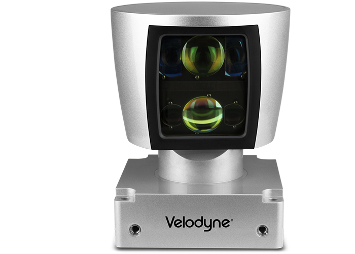
In this section, we will load a set of Lidar points from the file and display it from a top view perspective. Also, we will manually remove points that are located in the road surface. This is an important step which is needed to correctly compute the time-to-collision in the final project. The Lidar points have been obtained using a Velodyne HDL-64E sensor spinning at a frequency of 10Hz and capturing approximately 100k points per cycle. Further information on the KITTI sensor setup can be found here : http://www.cvlibs.net/datasets/kitti/setup.php

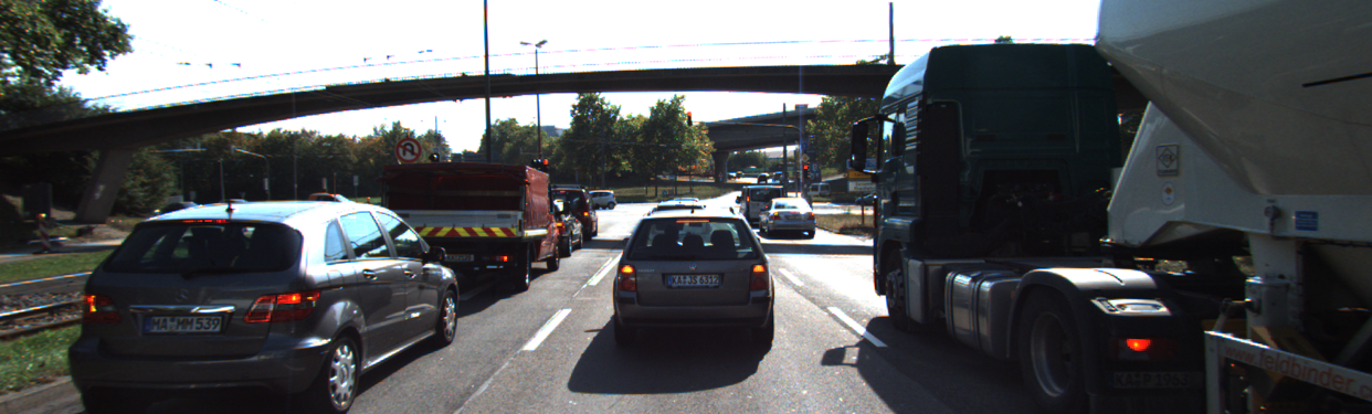
As will be detailed later, the Velodyne sensor has been synchronized with a forward-looking camera, which, at the time of capturing the Lidar data used in this section, was showing the following (by now very familiar) scene.

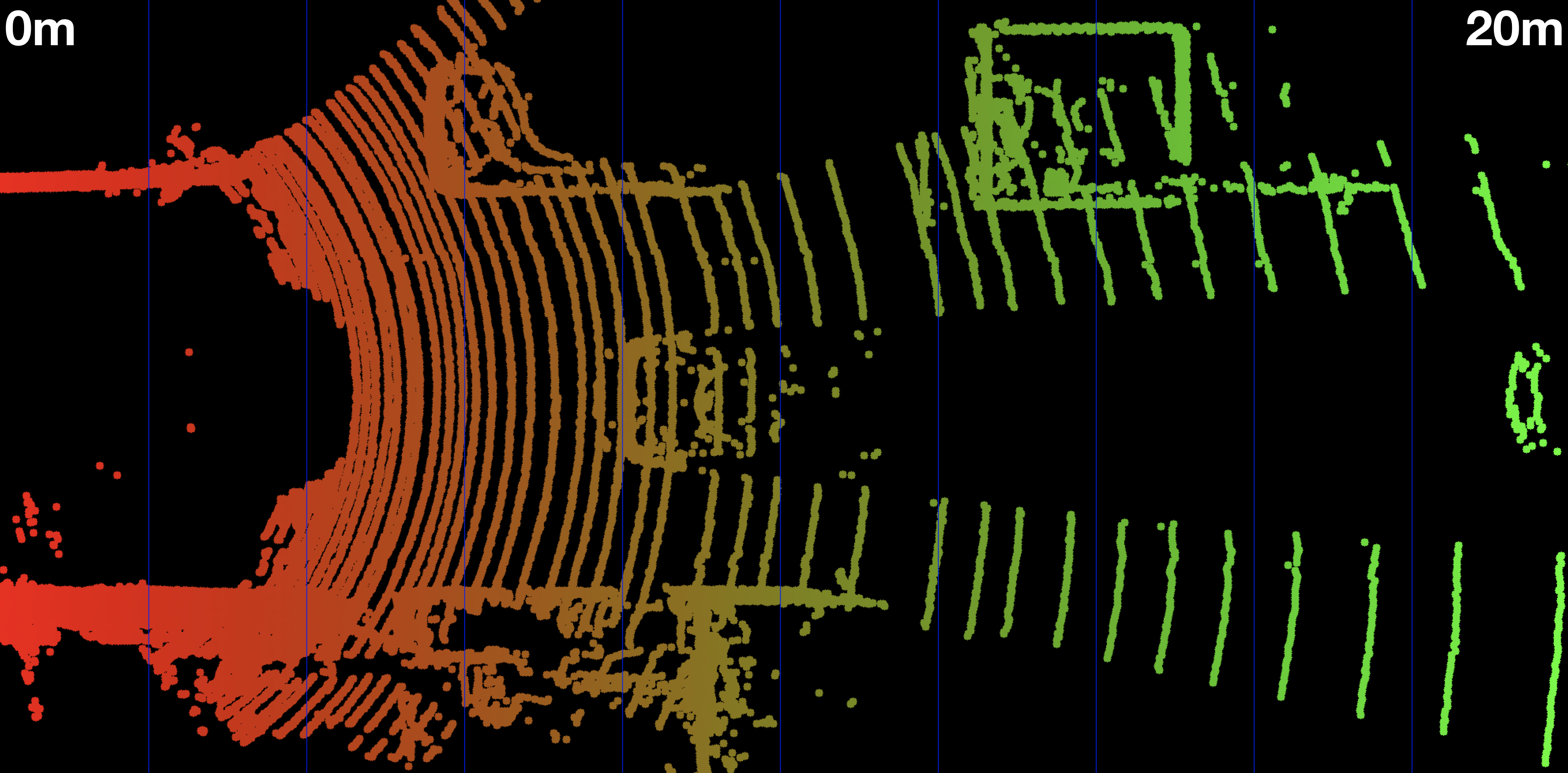
The Lidar points corresponding to the scene are displayed in the following figure, together with the Velodyne coordinate system and a set of distance markers. While the top view image has been cropped at 20m, the farthest point for this scene in the original dataset is at ~78m.

Exercise

The following code in show_lidar_top_view.cpp loads and displays the Lidar points in a top view perspective. When you run the code example, you will see that all Lidar points are displayed, including the ones on the road surface. Please complete the following exercises before continuing:

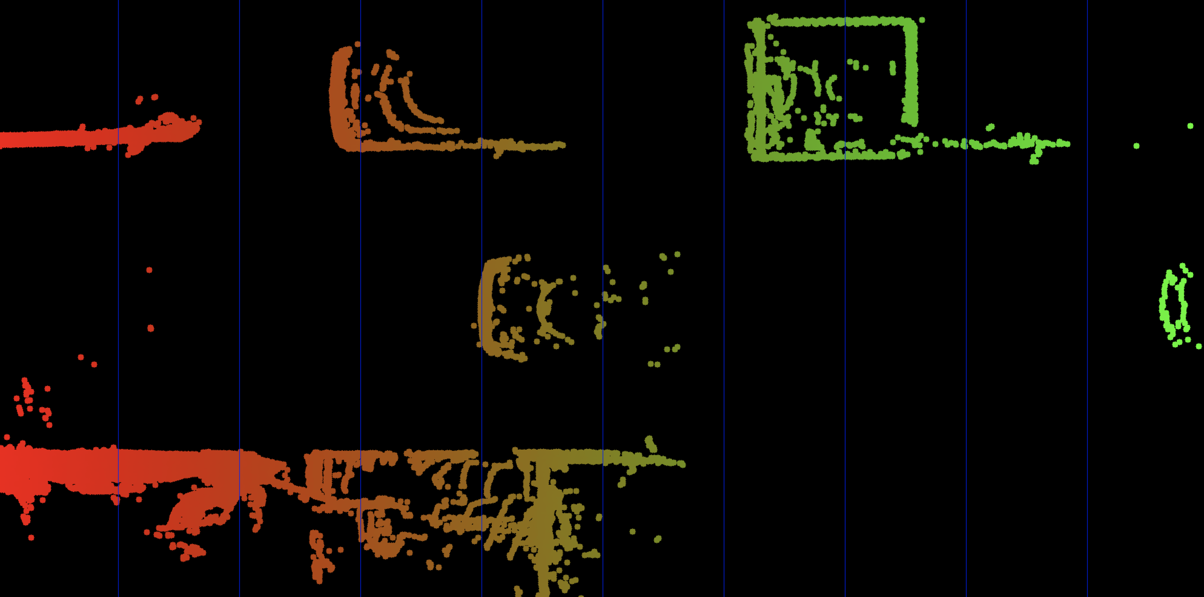
1. Change the color of the Lidar points such that X=0.0m corresponds to red while X=20.0m is shown as green with a gradual transition in between. The output of the Lidar point cloud should look like this:

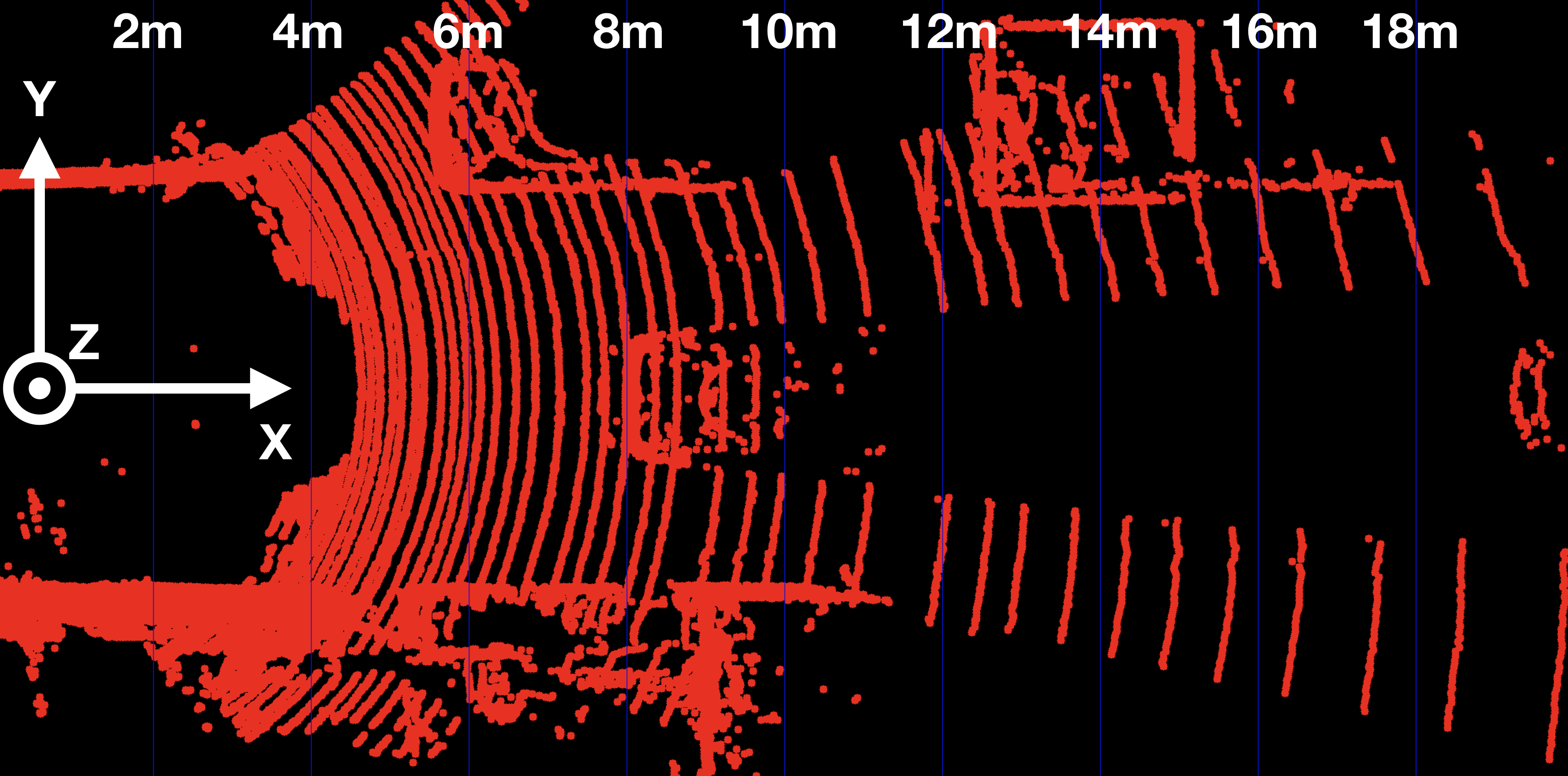
Remove all Lidar points on the road surface while preserving measurements on the obstacles in the scene. Your final result should look something like this:

Now that we can display Lidar data as 3D points in the sensor coordinate system, let us move on to the next section, where we want to start working on a way to project these points onto the camera image.

Merging Camera with Lidar Points

The easiest thing to do is to merge the 3D Lidar points into the camera image, but you need to make sure that:

• You synchronize all your lidar measurements to the exact recording time stamp of the camera

• If your camera is moving (that is typically the case for a robot), you compensate for that motion artifact. Because a typical lidar takes 100 ms to scan, and in that time you traveled a bit, and you need to compensate that motion so that the 3D point of the lidar falls exactly to the right pixel on the image.

Object Detection with YOLO

Until now, we are able to track 2D image features, measure 3D Lidar points and project them onto the image sensor. However, in order to achieve a stable TTC estimate in the final algorithm, it is not sufficient to observe single points. Instead, we need to cluster points that fall onto the same vehicle and discard those that are not relevant to our task (e.g. points on the road surface).

To do so, we need a way to reliably identify vehicles in our images and to place a bounding box around them. This section will introduce you to a deep-learning algorithm named YOLO (“You Only Look Once”) that is able to detect a range of various objects, including vehicles, pedestrians and several others. By the end of the section, you will be able to properly use the YOLO algorithm in your code for AI-based object detection.

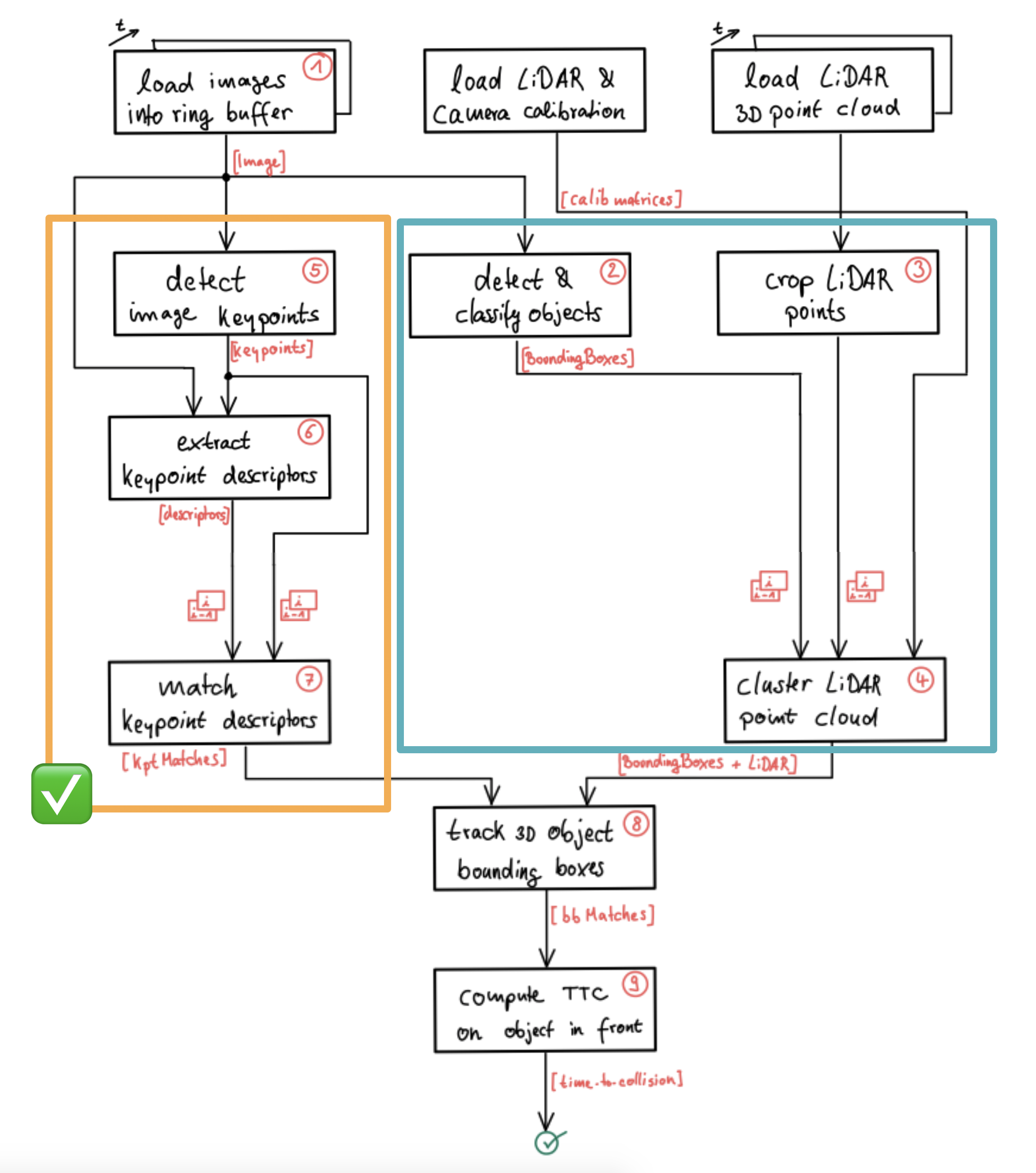
We need a way to detect vehicles in our images so that we can isolate matched keypoints as well as projected Lidar points and associate them to a specific object. Let us take a look at the program flow schematic we already discussed in the lesson on engineering a collision detection system.

Based on what you learned in the previous lesson, you are now able to detect and match keypoints using a variety of detectors and descriptors. In order to compute the time-to-collision for a specific vehicle however, we need to isolate the keypoints on that vehicle so that TTC estimation is not distorted due to the inclusion of matches on e.g. the road surface, stationary objects or other vehicles in the scene. One way to achieve this is to automatically identify the vehicles in the scene using object detection. The output of such an algorithm would (ideally) be a set of 2D bounding boxes around all objects in the scene. Based on these bounding boxes, we could then easily associate keypoint matches to objects and achieve a stable TTC estimate.

For the Lidar measurements, the same rationale can be applied. As you have learned in the previous course on Lidar, you already know that 3D points can be successfully clustered into individual objects, e.g. by using algorithms from the Point Cloud Library (PCL), which can be seen as an equivalent to the OpenCV library for 3D applications. In this section, let us look at yet another approach to group Lidar points into objects. Based on what you learned in the previous section, you now know how to project Lidar points onto the image plane. Given a set of bounding boxes from object detection, we could thus easily associate a 3D Lidar point to a specific object in a scene by simply checking whether it is enclosed by a bounding box when projected into the camera.

We will look in detail at both of the described approaches later in this section but for now, let us look at a way to detect objects in camera images - which is a prerequisite for grouping keypoint matches as well as Lidar points. in the schematic shown above, the content of the current lesson is highlighted by a blue rectangle and in this section we will be focussing on 'detecting & classifying objects‘.

Introduction into YOLO

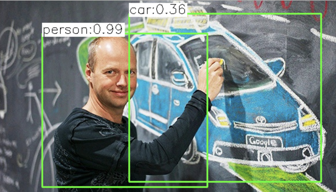
The aim of this section is to enable you to quickly leverage a powerful and state-of-the-art tool for object detection. It is not the purpose to perform a theoretical deep-dive into the inner workings of such algorithms, but rather you should be enabled to integrate object detection into the code framework of this course quickly and seamlessly. The following image shows the an example output of the code we will be developing in this section.

In the past, methods for object detection were often based on histograms of oriented gradients (HOG) and support vector machines (SVM). Until the advent of deep-learning, the HOG/SVM approach was long considered the state-of-the-art approach to detection. While the results of HOG/SVM are still acceptable for a large variety of problems, its use on platforms with limited processing speed is limited. As with SIFT, one of the major issues is the methods reliance on the intensity gradient - which is a costly operation.

Another approach to object detection is the use of deep-learning frameworks such as TensorFlow or Caffe. However, the learning curve for both is very steep and would warrant an entire course on its own. An easy-to-use alternative that works right out of the box and is also based on similar underlying concepts is YOLO, a very fast detection framework that is shipped with the OpenCV library. Developed by Joseph Redmon, Santosh Divvala, Ross Girshick, and Ali Farhadi at Cornell University, YOLO uses a different approach than most other methods: Here, a single neural network is applied to the full image. This network divides the image into regions and predicts bounding boxes and probabilities for each region. These bounding boxes are weighted by the predicted probabilities. The following figure illustrates the principle:

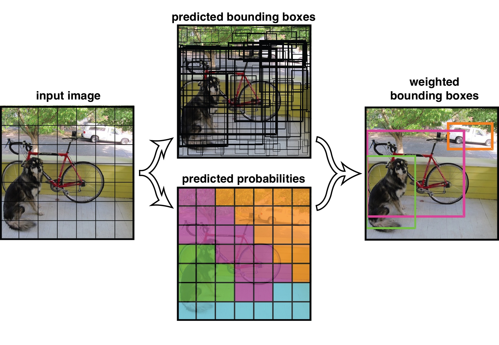
Other than classifier-based systems such as HOG/SVM, YOLO looks at the whole image so its predictions are informed by global context in the image. It also makes predictions with a single network pass unlike systems like R-CNN which require thousands of passes for a single image. This makes it extremely fast while at the same time generating similar results as other state-of-the-art methods such as the Single Shot MultiBox Detector (SSD).

The makers of YOLO have also made available a set of pre-trained weights that enable the current version YOLOv3 to recognize 80 different objects in images and videos based on COCO (http://cocodataset.org/#home) , which is a is large-scale object detection, segmentation, and captioning dataset. In the context of this course this means, that we can use YOLOv3 as an out-of-the-box classifier which is able to detect vehicles (and many other obstacles) with reasonable accuracy.

Standard CV vs Deep Learning

It still makes a lot of sense to learn the classical computer vision algorithms like half transforms, color spaces, edge detection. No everything has to be done with deep learning.

It is Okay to pre-train DNN with simulated data because you can just have a vast amount of data to pre-train. But, it is really hard to simulate the characteristics and noise models precisely to the chip that you want to have on your target vehicle. So, you will not get around with just training data in simulation. You will have to add annotated real data on the top.

Creating 3D-Objects

In this last section before the final project, you will learn how to combine 2D image features, 3D Lidar points and 2D YOLO-based vehicle bounding boxes to produce a stable 3D trajectory of a preceding vehicle. This will be the basis for creating a robust implementation of the TTC algorithm you have already learned about in a previous lesson.

Grouping Lidar Points Using a Region of Interest

The goal of this section is to group Lidar points that belong to the same physical object in the scene. To do this, we will make use of the camera-based object detection method we investigated in the last section. By using the YOLOv3 framework, we can extract a set of objects from a camera image that are represented by an enclosing rectangle (a "region of interest" or ROI) as well as a class label that identifies the type of object, e.g. a vehicle.

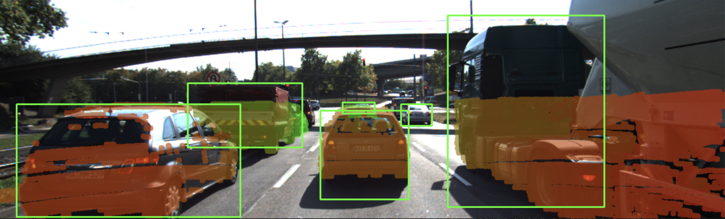
In the following, we will make use of the ROI to associate 3D Lidar points in space with 2D objects in the camera image. As can be seen in the following image, the idea is to project all Lidar points onto the image plane using calibration data and camera view geometry. By cycling through all Lidar points contained in the current data buffer in an outer loop and through all ROI in an inner loop, a test can be performed to check whether a Lidar point belongs to a specific bounding box.

If a Lidar point has been found to be within a ROI, it is added to the BoundingBox data structure we have seen in the previous section on object detection with YOLO. The BoundingBox structure introduced there now contains the following elements:

struct BoundingBox { // bounding box around a classified object (contains both 2D and 3D data)
int boxID; // unique identifier for this bounding box
int trackID; // unique identifier for the track to which this bounding box belongs

cv::Rect roi; // 2D region-of-interest in image coordinates
int classID; // ID based on class file provided to YOLO framework
double confidence; // classification trust

std::vector<LidarPoint> lidarPoints; // Lidar 3D points which project into 2D image roi
std::vector<cv::KeyPoint> keypoints; // keypoints enclosed by 2D roi
std::vector<cv::DMatch> kptMatches; // keypoint matches enclosed by 2D roi
};

During object detection, the members "boxID", "roi", "classID" and "confidence" have been filled with data. During Lidar point grouping in this section, the member "lidarPoints" is filled with all points within the boundaries of the respective ROI rectangle. In terms of the image shown above, this means that all colored Lidar points which have been projected into the camera image are associated with the green rectangle which encloses them. Lidar points not enclosed by a rectangle are ignored.

In some cases, object detection returns ROI that are too large and thus overlap into parts of the scene that are not a part of the enclosed object (e.g. a neighboring vehicle or the road surface). It is therefore advisable to adjust the size of the ROI slightly so that the number of Lidar points which are not physically located on the object is reduced. The following code shows how this can be achieved without much effort.

vector<vector<BoundingBox>::iterator> enclosingBoxes; // pointers to all bounding boxes which enclose the current Lidar point
for (vector<BoundingBox>::iterator it2 = boundingBoxes.begin(); it2 != boundingBoxes.end(); ++it2)
{
    // shrink current bounding box slightly to avoid having too many outlier points around the edges
    cv::Rect smallerBox;
    smallerBox.x = (*it2).roi.x + shrinkFactor * (*it2).roi.width / 2.0;
    smallerBox.y = (*it2).roi.y + shrinkFactor * (*it2).roi.height / 2.0;
    smallerBox.width = (*it2).roi.width * (1 - shrinkFactor);
    smallerBox.height = (*it2).roi.height * (1 - shrinkFactor);
}

By providing a factor "shrinkFactor '' which denotes the amount of resizing in [% ], a smaller box is created from the original bounding box. Further down in the code (see final project student code for details), a check is performed for each keypoint whether it belongs to the smaller bounding box. The figure below shows two different settings for "shrinkFactor". It can be seen that for the second figure, the projected Lidar points are concentrated on the central area of the preceding vehicle whereas Lidar points close to the edges are ignored.

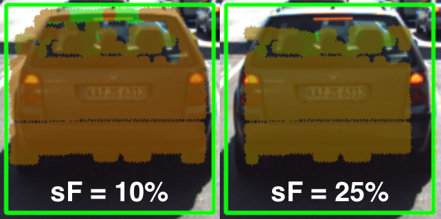
In practice, a moderate setting of 5-10% should be used to avoid discarding too much data. In some cases, when the bounding boxes returned by object detection are severely oversized, this process of boundary frame shrinkage can be an important tool to improve the quality of the associated Lidar point group.

Exercise: Avoiding Grouping Errors

Another potential problem in addition to oversized regions of interest is their strictly rectangular shape, which rarely fits the physical outline of the enclosed objects. As can be seen in the figure at the very top of this section, the two vehicles in the left lane exhibit a significant overlap in their regions of interest.

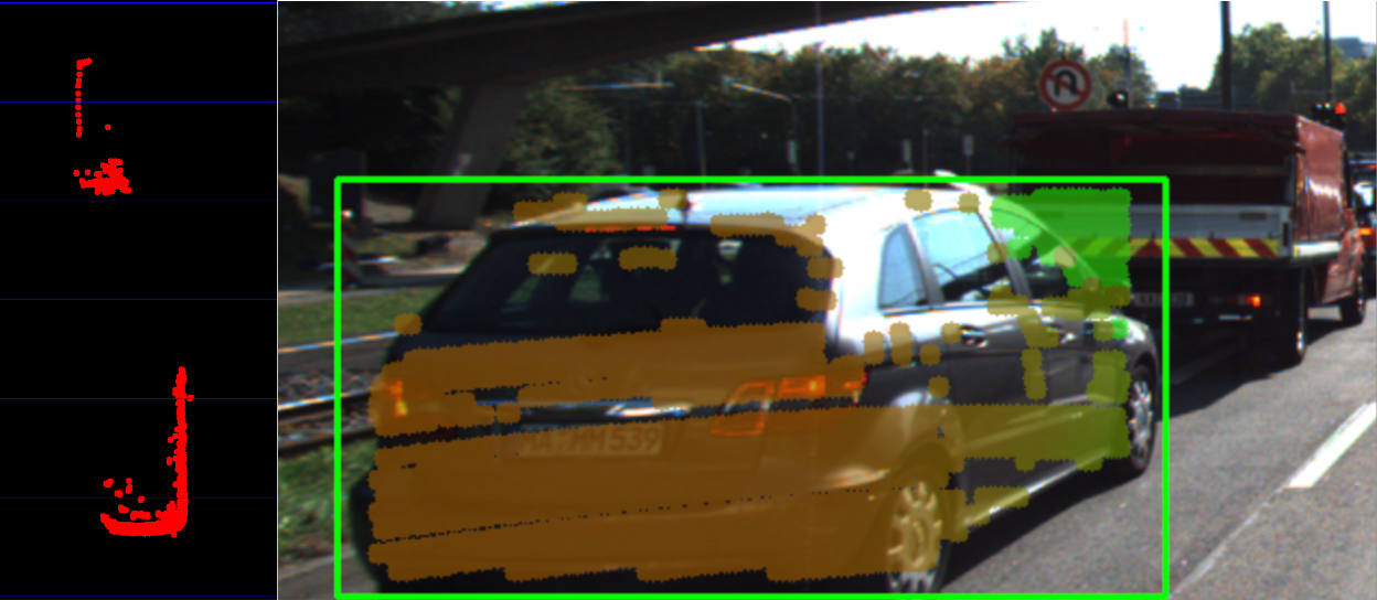
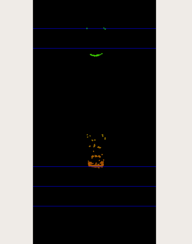
During point cloud association, Lidar points located on one vehicle might inadvertently be associated with another other vehicle. In the example illustrated in the figure below, a set of Lidar points in the upper right corner of the green ROI that actually belong to the red truck are associated with the blue vehicle. In the top view perspective on the left, this error becomes clearly visible.

In the following code example you will find the algorithm that is responsible for this incorrect behavior.

Your task now is to make changes to this code in such a way that Lidar points enclosed within multiple bounding boxes are excluded from further processing. We will lose some points but on the other hand you will get clean 3D objects.

You can find the code in the workspace below in cluster_with_roi.cpp, and after making, you can run the code using the executable cluster_with_roi.

• At the far end of scanning area, we do pick other points belonging to another vehicle into our bounding box. This is something we can't so easily avoid, at least not by image processing alone. We could run some algorithm on the lidar point cloud itself and look for spacial proximity.

Verify the Reliability of Sensor Fusion System

for everything that can go wrong, there must be a safety measure and a backup plan. Develop according to standards and code rules.

The sensor fusion module is right at the core and interacts with the rest of the robotic stack. You have upstream your perception modules and downstream your planning module. Sensor Fusion system have to be the component that brings everything together. You need to understand a lot about perception and how perception algorithms work, but you also have to understand the downstream applications of what is planning want to do with the data, how do you want to predict objects into the future. All of this has to be brought together in the right way.